Note: this document is now obsolete, following the introduction of the new California ISRM.
Patching the “Hole” in the California ISRM
The following page details the short-term solution to the current missing release height layer in the California ISRM. The future California ISRM that is in development will be trained on each release height and this patch will be removed.
Background
When the California ISRM was developed for the California Air Resources Board Contract 17RD0061, three release elevations were created:
- (L0) Ground level and low stack: below 57 m
- (L1) Medium and high stack: 57-140 m
- (L2) High elevation plumes: above 760 m
This results in a lack of estimates for emissions that occur between 140 and 760 meters, or the “hole”.
The US ISRM used for most of the published literature does not have this issue, so there is no peer-reviewed approach for solving this problem. As we develop the California ISRM, we can decide to avoid having this problem in the future, so this is a temporary (but important) problem.
What emissions sources even fall into this release height range?
- Airplane take-off and landing
- Rooftop building sources (e.g., rooftop generators)
- Some tall stacks
Temporary Solution
As noted above, the long-term solution for this issue is ensuring that the new ISRM for California includes reasonable layers for all near-surface release heights. Until then, ECHO-AIR takes the following approach.
In order to avoid overprescribing precision between 140 and 760 meters and slowing down ECHO-AIR’s processing, ECHO-AIR will do the following:
- Identify emissions that fall between L1 and L2.
- Notify the user about potential imprecision for sources that are released in this range.
- Perform a simple average of L1 and L2 to reasonably approximate ground-level concentrations from these source releases.
Brief Case Study and Justification for Solution
As a final note on this page, we performed a simple test of four potential solutions to the hole patching using California’s Cap-and-Trade facility emissions.
Emissions Release Height
The first test done here asks the question: what fraction of emissions from California’s Cap-and-Trade regulated facilities are released in the hole? We assigned layer labels to each reported emissions in the 2012 to 2017 Cap-and-Trade data and normalized by the total emissions of each pollutant.
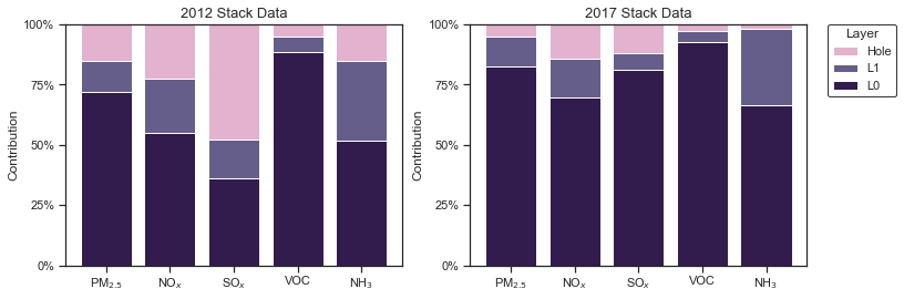
A few key takeaways:
- The hole accounted for less of the total emissions in 2017 than in 2012
- For primary PM2.5, which is most likely to affect nearby receptors, the hole is responsible for 4-15% of emissions.
- For emissions of the other four species, the hole was responsible for 14-22% of NOx, 2-5% of VOC, 12-48% of SOx, and 2-15% of NH3.
- SOx emissions in 2012 are an outlier, but as the low sulfur fuel laws continue, the emissions of SOx from these elevated staionary sources should decrease too.
Testing Four Strategies
The next test compares four potential strategies for patching the hole to bound the potential uncertainty with results. The four strategies are as follows:
- Assign to lower layer: In theory, the closer an emissions source is to the ground, the more likely it is to result in higher exposures near the source. This may be a more conservative approach.
- Use the higher of L1 and L2 for each cell: This is likely the most conservative approach. It will look at the row of the ISRM corresponding to the cell’s influence on receptors and pick the highest option between L1 and L2 for each receptor.
- Average L1 and L2 to create a middle “layer”: This is a simpler approach to the linear interpolation option. It still takes into account that impacts will be lower than L1 and higher than L2, but it doesn’t assign any artificial precision between.
- Assign to the upper layer: This should be the least conservative option, as impacts from the highest layer on the ground-level are the lowest.
The results of all four strategies are shown below for emissions in 2012 and 2017.
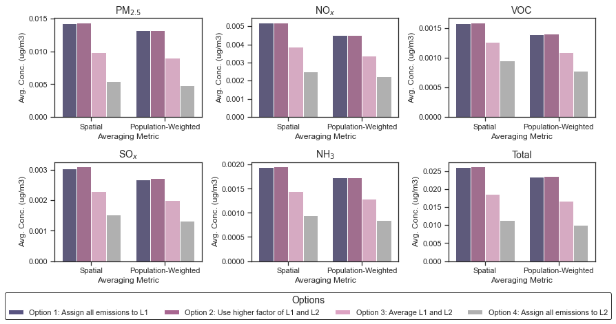
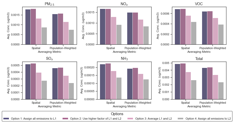
Based on these results, we are opting for Option 3 (Average L1 and L2) because it is the most reasonable middle-estimate between these bounds.
Testing ECHO-AIR
Finally, we look at the results of this choice by looking at the spatial patterns of impacts that result from emissions occurring in the hole, given the choice of averaging L1 and L2. We ran both (1) the full 2012 stack emissions and (2) all stack emissions occurring outside the hole through ECHO-AIR and substracted the differences. The spatial pattern in the San Francisco Bay Area is shown below. Sources that release in the hole are marked as small purple circles.
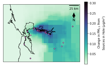
Additionally, it is useful to contextualize these results in the greater picture of population exposure. To do this, we compare the population-weighted means estimated from each of these scenarios as:
- Full stack PWM: 0.47 ug/m3
- Stack data minus the hole: 0.45 ug/m3